Harnessing GARCH Models in R for Advanced Time Series Forecasting

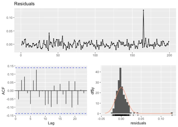
The newly introduced garchf package offers a friendly approach to GARCH modeling, tapping into the extensive capabilities of the underlying rugarch framework. By integrating this functionality into a familiar forecast-style interface, it allows users to generate, visualize, and assess GARCH-based forecasts effectively. The centerpiece of this package is the xgarchf() function, which enables the fitting of various GARCH models to univariate time series data.

Modeling Options and Output

The xgarchf() function supports a wide array of variance models, including the classic sGARCH, the exponential GARCH model (eGARCH), the GJR-GARCH variant (gjrGARCH), asymmetrical power GARCH (apARCH), and integrated GARCH (iGARCH). This variety allows users to select models that best capture the characteristics of their data. You'll also notice that users can specify several parameters, including ARMA order, GARCH order, and the distribution for errors, which adds a layer of customization to the modeling process. The output resembles standard forecast objects, featuring point forecasts, prediction intervals, and simulated future paths. This consistency with forecast objects makes it easier for seasoned statisticians and newcomers alike to interpret results.

Moreover, the flexibility of xgarchf() extends to probabilistic forecasting metrics. Users benefit from tools that compute sophisticated metrics like Continuous Ranked Probability Score (CRPS), pinball loss, and Winkler scores. Such metrics are vital for assessing model performance through cross-validation techniques. This focus on metrics can be particularly useful in financial contexts, where decision-makers must navigate the risks linked to forecast uncertainty.

Application Example: Analyzing Google Stock Prices

To illustrate the practical application of this package, let’s consider Google’s daily closing stock price returns. Financial analysts often scrutinize such data to gauge market behavior, and GARCH models provide insights into volatility. The first step involves calculating returns:

y <- diff(log(fpp2::goog200))

Next, we can fit various GARCH models to this data, which is critical for understanding how different model structures influence outcomes:

fit1 <- xgarchf(y, h = 20, model = "eGARCH")
fit2 <- xgarchf(y, h = 20, model = "sGARCH")
fit3 <- xgarchf(y, h = 20, model = "gjrGARCH")
fit4 <- xgarchf(y, h = 20, model = "iGARCH")

Reviewing the summaries of the fitted models offers statistical insights, deepening understanding. For instance:

print(summary(fitted(fit1)))

Each model presents its respective summary statistics, allowing for a comparative analysis across the fitted models. This step highlights the significance of model selection in forecasting. What this means for you as a practitioner is that understanding each model's nuance can inform better predictive accuracy and risk management, especially in volatile markets.

Cross-Validation Techniques

Evaluating the effectiveness of the GARCH model forecasts isn’t just a formality; cross-validation is essential for establishing model reliability. Here’s the thing: if your model can’t predict accurately outside of its training data, its practical usefulness is diminished. By employing the crossvalidation package, you can systematically compute evaluation metrics. These metrics can shed light on accuracy and reliability:

spl_m5 <- function(predicted, observed) {
    ...
}

The next step involves applying the cross-validation method to effectively gauge the performance of your models:

res <- crossvalidation::crossval_ts(
    y = y,
    initial_window = 150,
    horizon = 10,
    fixed_window = FALSE,
    fcast_func = garchf::xgarchf,
    eval_metric = eval_metric95,
    fit_params = list(arma_order=c(0, 0), garch_order = c(1, 1), model = "eGARCH", level=95),
    show_progress = FALSE
)

This method enables visualization of metrics such as Root Mean Square Error (RMSE), Mean Absolute Error (MAE), and coverage rates for a comprehensive comparison across models. The summary output captures these performance indicators succinctly. It serves as a snapshot of how well each model performs under cross-validation, which can be the deciding factor for users contemplating which model to use in practice.

Implications and Future Outlook

The emergence of the garchf package marks a significant advancement for statisticians and data scientists who require rigorous forecasting methods for financial and economic data. Embedding GARCH analysis into the user-friendly forecast interface streamlines workflows for practitioners everywhere, from academia to industry. Its implications for volatility forecasting are broad, given the perpetual uncertainty characterizing financial markets.

While the application showcased focuses on Google’s stock data, the true potential lies in the package’s adaptability to various time series. This adaptability opens avenues for further research and practice, from evaluating energy prices to assessing consumer behaviors, to the realm of cryptocurrency fluctuations. In sectors where volatility is a significant risk factor, the ability to forecast and visualize that volatility accurately has notable practical relevance. This means you'll want to keep an eye on developments in this area, as the evolution of packages like garchf can significantly impact how we approach time series forecasting in financial contexts.